Data sources used in csens.org
BP Statistical review of world energy
The World Bank Development Indicators
Ph and dissolved CO2 in the ocean surface water
Hadcrut and HadSST

Torungen lighthouse and weather station Norway
HadCRUT is the dataset of monthly instrumental temperature records formed by combining the sea surface temperature records compiled by the Hadley Centre of the UK Met Office and the land surface air temperature records compiled by the Climatic Research Unit (CRU) of the University of East Anglia.
The HadCRUT4 data are neither interpolated nor variance adjusted.
Hadley sea surface
The Met Office Hadley Centre's sea surface temperature data set, HadSST3 is a monthly global field of SST on a 5° latitude by 5° longitude grid from 1850 to date. The data have been adjusted to minimize the effects of changes in instrumentation throughout the record.Berkley Earth
Berkeley Earth is a Berkeley, California based independent non-profit focused on land temperature data analysis for climate science.
Berkeley Earth was founded in early 2010 with the goal of addressing the major concerns from outside the scientific community regarding global warming and the instrumental temperature.
Berkeley Earth's primary product is an analysis of summary air temperatures over land.
Berkeley Earth combines our land data with a modified
version of the HadSST ocean temperature data set. The result is a global average temperature data set.
Links to further info:
HADCRUT site,
HADCRUT4 source data,
HADSST site,
HADSST3 source data,
Berkley Earth, Land only site,
Berkley Earth, Land only source data,
Berkley Earth Land + Ocean site,
Berkley Earth Land + Ocean source data
Satellite observations
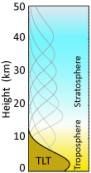
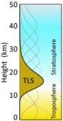
Two datasets are provided here; Temperature Lower Troposphere (TLT), and Temperature Lower Stratosphere (TLS).
TLT measures the temperatures from the surface up to approximately 10 km, with most weight in approximately 2.5 kilometer height as shown on the left figure below. TLS measures the altitudes from 10 to 30 km as shown in the right figure below.
|
|
Satellite observations from RSS
RSS is a private research company which processes microwave data from a variety of NASA satellites.
The monthly data files are used as source for these time series. Links to further info:
RSS site for upper air temperatures,
Satellite description from Nasa
RSS require that users register their email at the RSS site before providing access to the RSS source data.
The source files used here are:
RSS_Monthly_MSU_AMSU_Channel_TLT_Anomalies_Land_and_Ocean for the troposphere and
RSS_Monthly_MSU_AMSU_Channel_TLS_Anomalies_Land_and_Ocean for the stratosphere.
Satellite observations from University of Alabama in Huntsville (UAH)
The University of Huntsville publish monthly records for lower troposphere and lower stratosphere.The troposphere data can be downloaded here.
The stratosphere data can be downloaded here.
Weather Balloons
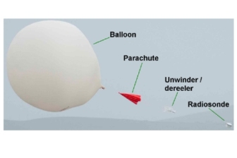
A radiosonde is a small expendable package of instruments which is carried aloft into the atmosphere below a hydrogen, or helium-filled, balloon. As the radiosonde ascends, measurements of temperature and relative humidity are made at 2 second intervals.
The balloon typically ascends at 5 m/s to reach a height of
about 25 km. As pressure decreases with height, the balloon expands until it bursts at which point the instrument package returns to earth borne by a parachute.
Radiosonde Atmospheric Temperature Products for Assessing Climate (RATPAC) are datasets created through a collaborative effort involving NOAA scientists from the Air Resources Laboratory, the Geophysical Fluid Dynamics Laboratory, and NCEI. Observations in the dataset are collected by hydrogen-filled weather balloons that carry a radiosonde up in the air to measure variables including temperature, humidity, and atmospheric pressure.
The RATPAC stations are a subset of the greater Radiosonde Archive of over 1,500 globally distributed stations. RATPAC data come from 85 stations with near-global coverage. The aim of the RATPAC series is to create time series from radiosonde temperatures that are less influenced by historical changes in instruments and measurement practices. Where available, data begin in 1958 and extend through the present.
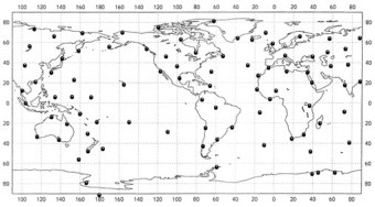 Global network of radiosonde stations
RATPAC station List
| NAME | Country | Latitude | Longitude | Elevation in meters |
|---|---|---|---|---|
| JAN MAYEN | Greenland sea | 70.93 | -8.67 | 9 |
| SODANKYLA | Finland | 67.37 | 26.65 | 178 |
| LERWICK | UK | 60.13 | -1.18 | 84 |
| KEFLAVIK | Iceland | 63.97 | -22.6 | 54 |
| AMMASSALIK | Greenland | 65.6 | -37.63 | 52 |
| GIBRALTAR | Gibraltar | 36.15 | -5.35 | 4 |
| LAJES/SANTA RITA | Portugal | 38.73 | -27.07 | 112 |
| MUENCHEN | Germany | 48.25 | 11.55 | 489 |
| OSTROV PREOBR. | Russia | 74.67 | 112.93 | 60 |
| OSTROV CHETYR. | Russia | 70.63 | 162.4 | 38 |
| PECHORA | Russia | 65.12 | 57.1 | 56 |
| TURUKHANSK | Russia | 65.78 | 87.95 | 37 |
| VERKHOYANSK | Russia | 67.55 | 133.38 | 137 |
| OMSK | Russia | 54.93 | 73.4 | 91 |
| KIRENSK | Russia | 57.77 | 108.12 | 257 |
| PETROPAVLOVSK | Russia | 53.02 | 158.72 | 78 |
| ROSTOV | Russia | 47.25 | 39.82 | 78 |
| CHKALOV | Russia | 51.75 | 55.1 | 119 |
| ASHKHABAD | Turkmenistan | 37.97 | 58.33 | 304 |
| BET DAGAN | Israel | 32 | 34.82 | 35 |
| JEDDAH/ABDUL AZIZ AIRPORT | Saudi Arabia | 21.7 | 39.18 | 17 |
| KING'S PARK | China | 22.32 | 114.17 | 66 |
| WAKKANAI | Japan | 45.42 | 141.68 | 11 |
| KAGOSHIMA | Japan | 31.63 | 130.6 | 31 |
| MARCUS IS. | Japan | 24.3 | 153.97 | 9 |
| BANGKOK | Thailand | 13.73 | 100.57 | 20 |
| SINGAPORE/CHANGI | Singapore | 1.37 | 103.98 | 3 |
| KASHI | China | 39.47 | 75.98 | 1291 |
| MINQIN | China | 38.72 | 103.1 | 1367 |
| SANTA CRUZ DE TENERIFE | Spain | 28.45 | -16.25 | 36 |
| NIAMEY-AERO | Niger | 13.48 | 2.17 | 227 |
| DAKAR/YOFF | Senegal | 14.73 | -17.5 | 27 |
| ASCENSION IS./WIDEAWAKE | St. Helena | -7.97 | -14.4 | 79 |
| DIEGO GARCIA | Br. Indian Oc. Terr. | -7.3 | 72.4 | 3 |
| MARTIN DE VIVIES | French S. Antarctic | -37.8 | 77.53 | 29 |
| TRIPOLI AIRPORT | Libya | 32.67 | 13.15 | 82 |
| NAIROBI/DAGORETTI | Kenya | -1.3 | 36.75 | 1798 |
| ABIDJAN | Cote D'Ivoire | 5.25 | -3.93 | 8 |
| ANTANANARIVO/IVATO | Madagascar | -18.8 | 47.48 | 1276 |
| DURBAN AIRPORT | South Africa | -29.97 | 30.95 | 14 |
| CAPE TOWN AIRPORT | South Africa | -33.97 | 18.6 | 42 |
| GOUGH IS. | South Africa | -40.35 | -9.88 | 54 |
| MARION IS. | South Africa | -46.88 | 37.87 | 21 |
| BARROW | USA | 71.3 | -156.78 | 12 |
| ST. PAUL ISLAND | USA | 57.15 | -170.22 | 10 |
| ANNETTE ISLAND | USA | 55.03 | -131.57 | 37 |
| MOULD BAY | Canada | 76.23 | -119.32 | 58 |
| ALERT | Canada | 82.5 | -62.33 | 66 |
| ST. JOHNS | Canada | 47.67 | -52.75 | 140 |
| MOOSONEE | Canada | 51.27 | -80.65 | 10 |
| BAKER LAKE | Canada | 64.3 | -96 | 49 |
| BROWNSVILLE | USA | 25.92 | -97.42 | 7 |
| SAN DIEGO | USA | 32.85 | -117.12 | 132 |
| DODGE CITY | USA | 37.77 | -99.97 | 791 |
| GREAT FALLS | USA | 47.46 | -111.38 | 1130 |
| BERMUDA NAS KINDLEY | Bermuda | 32.37 | -64.68 | 40 |
| SAN JUAN | Puerto Rico | 18.43 | -66 | 19 |
| BOGOTA/EL DORADO | Columbia | 4.7 | -74.15 | 2546 |
| MANAUS | Brazil | -3.15 | -59.98 | 84 |
| GALEAO | Brazil | -22.82 | -43.25 | 6 |
| ANTOFAGASTA | Chile | -23.42 | -70.47 | 137 |
| ISLA DE PASCUA | Chile | -27.13 | -109.47 | 47 |
| PUERTO MONTT | Chile | -41.43 | -73.1 | 90 |
| BUENOS AIRES/EZEIZA AERO | Argentina | -34.82 | -58.53 | 20 |
| AMUNDSEN-SCOTT | Antarctica | -90 | 0 | 2835 |
| BELLINGSHAUSEN | Antarctica | -62.2 | -58.93 | 16 |
| SYOWA | Antarctica | -69 | 39.58 | 15 |
| MOLODEZNAJA | Antarctica | -67.67 | 45.85 | 40 |
| MAWSON BASE | Antarctica | -67.6 | 62.88 | 15 |
| MCMURDO | Antarctica | -77.85 | 166.67 | 24 |
| HILO/LYMAN | USA | 19.72 | -155.07 | 10 |
| CHUUK | Micronesia | 7.47 | 151.85 | 3 |
| MAJURO ATOLL | Marshall Islands | 7.08 | 171.38 | 3 |
| KOROR | Palau | 7.33 | 134.48 | 30 |
| HONIARA | Solomon Islands | -9.42 | 160.05 | 56 |
| NADI AIRPORT | Fiji | -17.75 | 177.45 | 25 |
| TAHITI-FAAA | French Polynesia | -17.55 | -149.62 | 2 |
| INVERCARGILL | New Zealand | -46.42 | 168.32 | 4 |
| CHATHAM ISLAND | New Zealand | -43.95 | -176.57 | 49 |
| DARWIN | Australia | -12.43 | 130.87 | 29 |
| TOWNSVILLE | Australia | -19.25 | 146.77 | 9 |
| PERTH AIRPORT | Australia | -31.93 | 115.97 | 20 |
| ADELAIDE AIRPORT | Australia | -34.95 | 138.53 | 4 |
| NORFOLK ISLAND | Norfolk Island | -29.03 | 167.93 | 110 |
| MACQUARIE ISLAND | Australia | -54.5 | 158.95 | 8 |
Links to further info:
NOAA Weather balloon,
Weather balloon description from the UK Met Office,
Temporal Homogenization of Monthly Radiosonde Temperature Data. Part I: Methodology,
RATPAC-A Raw data,
RATPAC-B Raw data
Sea level gauges
Traditionally, global sea level change has been estimated from tide gauge measurements collected over the last century. Tide gauges, usually placed on piers, measure the sea level relative to a nearby geodetic benchmark. The most commonly used tide gauge measurement system is a float operating in a stilling well. Surveys of the tide gauge site are performed regularly to account for any settling of the site.
Major conclusions from tide gauge data have been that global sea level has risen approximately 10-25 cm during the past century.
The first gauge series is based on a selection made by Church and White, referenced below.
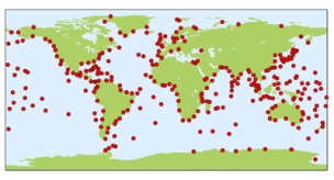
Global Sea Level Observing System (Gloss) is a network of 290 globally distributed coastal tide gauge stations.
The available selections for Gloss are:
- Simple Global average
- This is a simple average of all stations
- Gridded Global average
- The grid is 10-degree latitude x 10-degree longitude, i.e. an 18 times 36 grid over the globe. The stations are first averaged in each grid-cell, then the globe average is taken by averaging the grid-cells.
- Long series
- This is series at least 75 years long and continuing to at least two years before current.
- Extra Long series
- This is series at least 100 years long and continuing to at least two years before current.
- 60N to NP
- 60-degree North to North Pole. 60N is the latitude of Hudson Bay, Oslo, Stockholm, Helsinki and the South of Alaska.
- Equator to 60N
- Most of the stations are located in this sector
- Equator to 60S
- Similar for Southern hemisphere.
- 60S to SP
- 60 degrees south to the South Pole. 60S is the latitude of the Northernmost tip of the Antarctic continent. All the globes inhabited continents and islands are located north of 60S.
Links to further info about the data from sea level gauges:
CSIRO Austalia,
A list of the tide gauges used for constructing the time series(zipped),
Church, J.A., White, N.J., 2011. Sea-Level Rise from the Late 19th to the Early 21st Century.
Surveys in Geophysics, Volume 32 ,
Gauges data file (zipped),
List of gauge stations with data.
Sea level satellite altimetry
Sea level by Satellite Altimetry
A series of satellite missions that started with TOPEX/Poseidon (T/P) in 1992 and continued with Jason-1 (2001 - 2013)
and Jason-2 (2008 - present) estimate global mean sea level every 10 days with an uncertainty of 3 - 4 mm.,
Links to further info about the data from sea level by satellite altimetry:
-
NOAA Laboratory for Satellite Altimetry,
-Data download site,
The chosen dataset is 'Topex, Jason-1, Jason-2 seasonal signal retained':
Source datafile
BP Statistical review of world energy
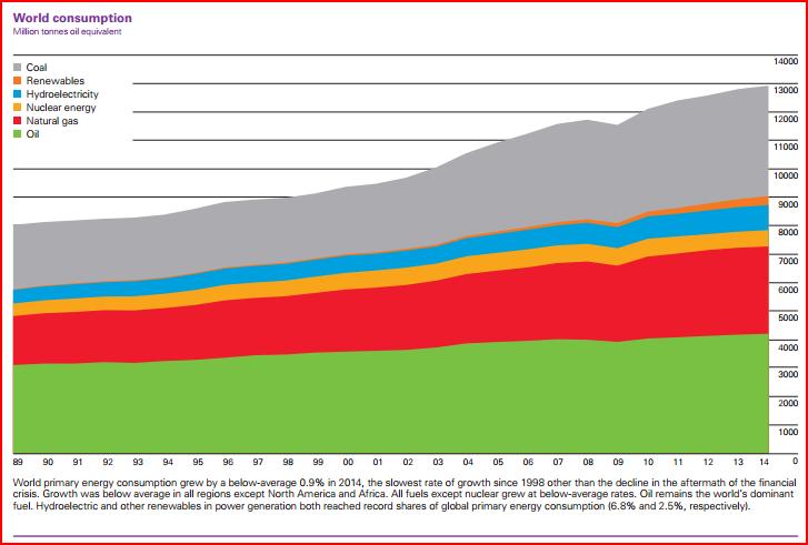
Since 1951, BP has annually published its Statistical Review of World Energy, which is considered an energy industry benchmark.
The presented statistics contains total CO2 emissions, total energy consumption and energy consumption for each major energy source.
all energy units are converted to Million tons oil equivalents (Mtoe).
1 million tons oil equivalent converts to:
1.11 billion cubic meters Natural gas
0.82 million tons Liquid Natural gas
1.5 million tons of hard coal
3 million tons of lignite
4.4 Terawatt-hours electricity. (Converted on the basis of thermal equivalence assuming 38% conversion efficiency in a modern thermal power station.
Thermal energy equivalence is 12 Terawatt-hours.)
Links to further info:
BP Statistical Review of World Energy,
Full report 2018
Data source
The World Bank Development Indicators
The primary World Bank collection of development indicators, compiled from officially-recognized international sources. It presents the most current and accurate global development data available, and includes national, regional and global estimates.
A few indicators which are relevant for energy production, climate gas emissions, and global air pollution, are presented here.
| Label | Explantion |
|---|---|
| Population | Total number of living citizens all ages |
| Life-expectancy-at-birth | Average number of years that a newborn is expected to live if current mortality rates continue to apply. |
| Mortality rate infant | Number of deaths under 1 year age per 1000 live births |
| Mortality rate under-5 | Number of deaths under 5 years age per 1000 live births |
| Fertility rate | Births per woman. The average number of children that would be born to a woman over her lifetime if the woman were to experience the current age-specific fertility rates through her reproductive years and were to survive from birth through the end of her reproductive life (to age 49) |
| Youth. Fertilit. (ages 15-19) | Adolescent fertility rate (births per 1000 women ages 15-19) |
| Contraceptive prevalence (% wom. 15-49) | Contraceptive prevalence any methods (% of women ages 15-49) |
| Male births per female births | Sex ratio at birth (male births per female births) |
| Literacy rate | Literacy rate adult total (% of people ages 15 and above) |
| Children out of school % | Percentage of children of primary school age out of school |
| Youth out of school % | Adolescents out of school (% of lower secondary school age) |
| Youth not in education or empl. % | Share of youth not in education, employment or training |
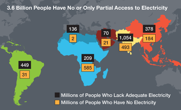
| Access to electricity | Percentage of population with access to electricity in their home |
| Open defecation % | Percentage of population practicing open defecation (no toilet, neighter WC nor privy) |
| At least basic sanitation % | The percentage of people using improved sanitation facilities that are not shared with other households. This indicator encompasses both people using basic sanitation services as well as those using safely managed sanitation services. Improved sanitation facilities include flush/pour flush to piped sewer systems, septic tanks or pit latrines; ventilated improved pit latrines, compositing toilets or pit latrines with slabs. |
| At least basic drinking w. serv. % | The percentage of people using basic water services as well as those using safely managed water services. Basic drinking water services is defined as drinking water from an improved source, provided collection time is not more than 30 minutes for a round trip. Improved water sources include piped water, boreholes or tubewells, protected dug wells, protected springs, and packaged or delivered water. |
| Safe drinking water serv. % | The percentage of people using drinking water from an improved source that is accessible in homes, available when needed and free from faecal and priority chemical contamination. Improved water sources include piped water, boreholes or tubewells, protected dug wells, protected springs, and packaged or delivered water. |
| Poverty ratio at $1.90 a day | Poverty headcount ratio at $1.90 a day, purchase power parity, constant 2011 US dollar |
| Poverty ratio $3.20 a day | Poverty headcount ratio at $3.20 a day, purchase power parity, constant 2011 US dollar |
| GDP (constant 2010 US$) | GDP total, in exchange rates, constant 2010 US dollar |
| GDP per capita PPP | GDP per capita purchase power parity, constant 2011 US dollar |
| Net foreign assets (current LCU) | Net foreign assets (current Local Currency Units) |
| Employment ratio | Employment to population ratio of population ages 15 and up who work for pay or profit for at least one hour per week(modeled ILO estimate) |
| Labor participation | Rate of labor force who work for pay or profit for at least one hour a week (% of total population ages 15-64) (modeled ILO estimate) |
| Unemployment | Unemployed people are those who report that they are without work, that they are available for work and that they have taken active steps to find work in the last four weeks. (% of total labor force) (modeled ILO estimate) |
| Part time employment | Percentage of workforce working less than 30 hours per week |
| Homicides (per 100 000 people) | Intentional homicides (per 100 000 people) |
| Traffic deaths | Mortality caused by road traffic injury (per 100 000 people) |
| Corruption rating(1=low to 6=high) | CPIA transparency accountability and corruption in the public sector rating (1=low to 6=high) |
| Forest area (sq. km) | Forest area (sq. km) |
| Agricultural land % | Agricultural land is land including arable land, land under permanent crops and land under permanent meadows and pastures. (% of land area) |
| Arable land % | Land able to be plowed (% of land area) |
| Cereal yield | Cereal yield (kg per hectare) |
| Crop production index | Crop production index (2004-2006 = 100) |
| PM2.5 air pollution | PM2.5 air pollution mean annual exposure (micrograms per cubic meter) |
| CO2 per capita | CO2 emissions per capita in metric tons (1000 kg). |
Links to further info:
The World Bank Development Indicators
Online database search engine
Data themes
Data source (zipped)
Sea Ice
Both Arctic and Antarctic sea ice varies considerably during the annual cycle as shown below

climate4you.com – Ole Humlum – Professor, University of Oslo Department of Geosciences – Click the pic to view at source
The trends over the last decades are that the arctic ice has been declining, and the Antarctic ice has a small increase.
The overall trend is a declining ice coverage.
Links to further info: Links to further info: Strong acids have a low Ph value. Vinegar has a Ph of approximately 2.2, and sulfuric acid (battery acid) has a Ph of 1.0.
Ammonia on the other hand has a Ph of 11.0 and is therefore an example of a strong alkaline solution. The mean pH of ocean waters ranges between 7.5 and 8.4 in the open ocean,
which means that the ocean is a mildly alkaline solution.
Ocean acidification can also be caused by other chemical additions or subtractions from the oceans that are natural (e.g., increased volcanic activity, methane hydrate releases,
long-term changes in net respiration) or human-induced (e.g., release of nitrogen and sulfur compounds into the atmosphere). Anthropogenic ocean acidification refers to the
component of pH reduction that is caused by human activity.
Data download directory,
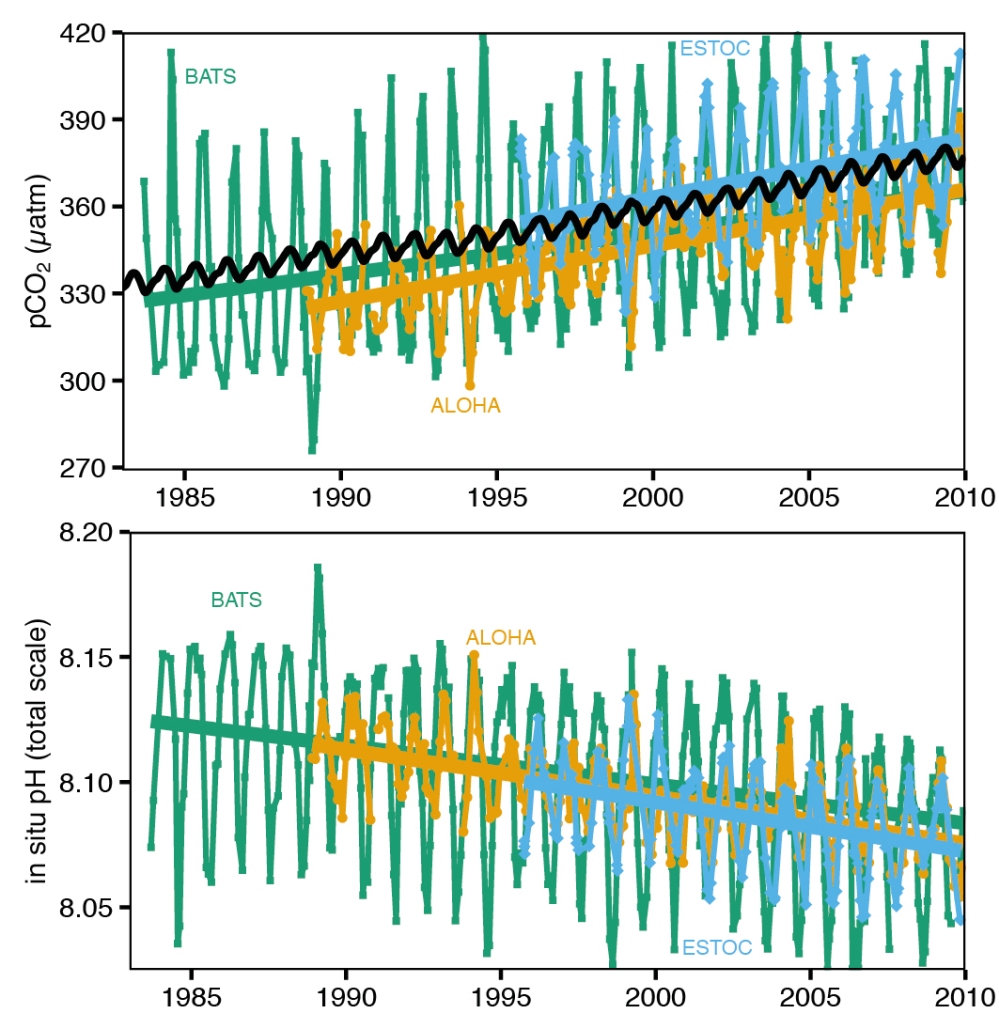
Ph and dissolved CO2 in the ocean surface water
The Ocean PH data and dissolved CO2 data series are from the Hawaii Ocean Time-series (HOT) program and the Bermuda Atlantic Time-series study.
The Bermuda series goes back to 1983, and the HOT series start in 1988.
 Scientists working on the Hawaii Ocean Time-series (HOT)
program have been making repeated observations of the hydrography, chemistry and biology of the water column at a station north of Oahu, Hawaii since October 1988.
The objective of this research is to provide a comprehensive description of the ocean at a site representative of the North Pacific subtropical gyre.
Scientists working on the Hawaii Ocean Time-series (HOT)
program have been making repeated observations of the hydrography, chemistry and biology of the water column at a station north of Oahu, Hawaii since October 1988.
The objective of this research is to provide a comprehensive description of the ocean at a site representative of the North Pacific subtropical gyre.
The potential for acquiring more diverse and detailed time-series
data was a key motivator in allowing BIOS to establish the Bermuda Atlantic Time-series Study. The BATS team is involved in making monthly measurements of important
hydrographic, biological and chemical parameters throughout the water column at sites within the Sargasso Sea
Bermuda Atlantic Time-Series Study
Hawaii Ocean Time-series (HOT)
Bermuda source data
Hawaii source dataMore about Ph
Ph is a measure of acidity and alkalinity in a solution. Pure water at 25 degrees Celsius has a Ph of 7 and is defined as neutral. A Ph below 7 is considered 'acidic' and a Ph above 7
is considered 'alkaline' or 'basic'.
Note that pH also depends on temperature. Pure wate is only neutral at 25 °C and it decreases with increasing temperature.
For instance at 0 °C the pH of pure water is 7.47, and at 100 °C it's 6.14.

CO2 dissolves in water and the dissolved CO2 forms a weak acid (H2CO) which contribute to lowering the ocean Ph.
This process is called 'ocean acidification' although the ocean water is far from being pushed over from alkalinity to acidity, but it moves in the direction of acidity.
Link to further info:
According to IPCC (referenced below) the average pH of ocean surface waters has already fallen by about 0.1 units,
from about 8.2 to 8.1 (total scale), since the beginning of the industrial revolution.
The figure to the right show the connection between increased CO2 level and lowered Ph measured in the ocean surface water. Click for larger image.
IPCC AR 5 Chapter 3
More about the the oceans role in the carbon cycle
Since the beginning of the industrial era, the release of CO2 from industrial and agricultural activities has resulted in atmospheric CO2 concentrations that have increased from approximately 280 ppm to about 400 ppm in 2016. The oceans have absorbed approximately 165 PgC from the atmosphere over the last two and a half centuries. This means that about 40% of the man made CO2 emission has been absorbed by the oceans.
The oceans contain approximately 50 times as much carbon as the atmosphere, see figure above.
The rate of carbon uptake depends on the atmospheric CO2 level, the surface waters CO2 level, and the surface water temperature.
Cold water absorbs more CO2 than warm water. The relation between temperature and CO2 solubility in water is called Henry's Law. This relation has led to the question of whether the increased atmospheric CO2 level could have been caused by increased ocean temperature, and not the other way around.
However, Henry's law states that the atmospheric CO2 content should only raise by 12 ppm for each 1 Celsius increase in ocean temperature.
Since the atmospheric CO2 increase is ten times bigger than the relation described by Henry's law, the increase cannot have been caused by that alone.
Link to further info:
IPCC AR5 Chapter 6
Description of correlation between atmospheric CO2 content and temperature from the Vostoc ice cores:
S. Torn, Harte, GEOPHYSICAL RESEARCH LETTERS, VOL. 33, L10703"
Atmospheric CO2
The atmospheric CO2 series presented are Global marine surface, the Mauna Loa observatory in Hawaii, and the South Pole observatory. The Mauna Loa has recordings since 1958 and the South Pole data are from 1975.
The data are provided by The US National Oceanic and Atmospheric Administration (NOAA).
The Mauna loa primary observing site is located at the 3397 m (11,141 ft) level on Mauna Loa's north slopes.
The South Pole observatory is located at the geographical South Pole, 2837 m above sea level.

The Amundsen - Scott base, South Pole
Links to further info:
Mauna loa observatory
South Pole observatory
Global source data
Mauna Loa source data
South Pole source data
More about the carbon cycle
Carbon dioxide is an integral part of the carbon cycle, in which carbon is exchanged between the Earth's oceans, soil, rocks and biosphere.A simplified schematic of the global carbon cycle is shown below. The figure is from IPCC AR5",

Numbers represent reservoir mass, also called 'carbon stocks' in PgC (1 PgC = 1 billion tons C) and annual carbon exchange fluxes (in PgC per year). Black numbers and arrows indicate reservoir mass and exchange fluxes estimated for the time prior to the Industrial Era, about 1750.
The sediment storage is a sum of 150 PgC of the organic carbon in the mixed layer and 1600 PgC of the deep-sea CaCO3 sediments available to neutralize fossil fuel CO2.
Red arrows and numbers indicate annual 'anthropogenic' fluxes averaged over the 2000-2009 time period. These fluxes are a perturbation of the carbon cycle during
industrial era post 1750. These fluxes (red arrows) are:
Fossil fuel and cement emissions of CO2,
Net land use change, and
the Average atmospheric increase of CO2 in the atmosphere, also called 'CO2 growth rate'.
The uptake of anthropogenic CO2 by the ocean and by terrestrial ecosystems, often called 'carbon sinks' are the red arrows part of Net land flux and Net ocean flux.
Red numbers in the reservoirs denote cumulative changes of anthropogenic carbon over the Industrial Period 1750-2011. By convention, a positive cumulative change means that a reservoir has gained carbon since 1750
Atmospheric CH4 (Methane)
The atmospheric CH4 series presented are Global marine surface, the Mauna Loa observatory in Hawaii, and the South Pole observatory. The methane goes back to 1983.
The data are provided by The US National Oceanic and Atmospheric Administration (NOAA).
The Methane data comes from the same stations in Mauna Loa, Hawaii and South Pole base as the atmospheric CO2 data.
The Amundsen - Scott base front
Links to further info:
Mauna loa observatory,
South Pole observatory,
Global source data,
Mauna Loa source data,
South Pole source data
More about Methane
Methane (CH4) absorbs infrared radiation relatively stronger per molecule compared to CO2. On the other hand, the methane lifetime is less than 10 years in the troposphere as opposed to the very long lifetime of CO2.City Pollution
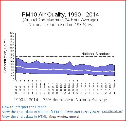
Data sources for city pollution are the US Environment Protection Agency (EPA) and Kings College UK.The time series for city pollution are single measurement stations. For cities with several measurements stations the station with the most complete recording has been chosen.
The measurements are not suitable for comparisons of the pollution level between different cities, since some measurement stations are located in city centers, and others in the city's surroundings. However, the measurements are well suitable for seeing the development over time. | ||||||||||||||||||||||
Stations used for Nitrogen Dioxide, PM10 and SO2:
| ||||||||||||||||||||||
Stations used for PM2.5:
| ||||||||||||||||||||||
The overall trends for PM and NO2 are shown below
| ||||||||||||||||||||||
Links to further info: |
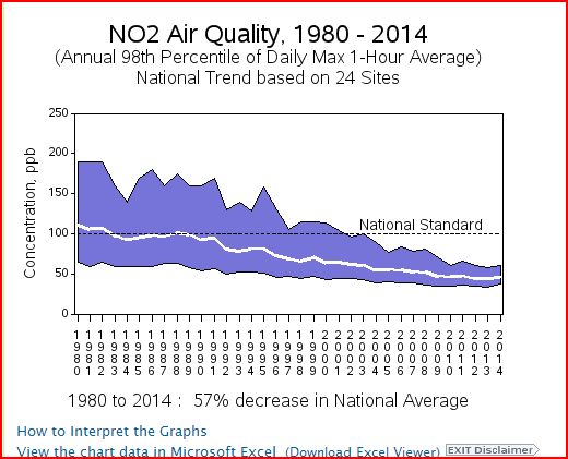
More about NO2
Nitrogen dioxide (NO2), is not to be confused with nitrous oxide (N2O). Nitrogen dioxide is a major local pollutant, but has a short lifetime of approximately 1 day in the atmosphere, depending on temperature and sunlight. Nitrous oxide, on the other hand, has a lifetime in the atmosphere of 114 years and is a greenhouse gas.Using a nationwide network of monitoring sites, EPA has developed ambient air quality trends for nitrogen dioxide (NO2), and particle pollution, also called Particulate Matter (PM). Under the Clean Air Act, EPA sets and reviews national air quality standards. Air quality monitors measure concentrations of NO2 and PM throughout the country.
Nasa Ceres
CERES is an acronym for Clouds and the Earth’s Radiant Energy Systems CERES products include both solar-reflected and Earth-emitted radiation from the top of the atmosphere to the Earth's surface. The CERES products used in Csens.org are:- Observed Top of the Atmosphere Shortwave Flux, All-sky conditions. This is outgoing shortwave flux.
- Observed Top of the Atmosphere Shortwave Flux, Clear-sky conditions This is outgoing shortwave flux assuming clear sky.
- Observed Top of the Atmosphere Longwave Flux, All-sky conditions This is outgoing longwave flux
- Observed Top of the Atmosphere Longwave Flux, Clear-sky conditions. This is outgoing longwave flux assuming clear sky.
- Observed Top of the Atmosphere Net Flux, All-sky conditions This is the net planetary flux. Positve values means net incoming flux, negative values means net outgoing flux.
- Observed Top of the Atmosphere Net Flux, Clear-sky conditions
- Observed Top of the Atmosphere Albedo, All-sky conditions This is also called the "Planetary_albedo"
- Observed Top of the Atmosphere albedo, Clear-sky conditions This is also called "Surface albedo"
- Observed Top of the Atmosphere Solar Insolation Flux, All-sky conditions This is the incoming shortwave flux from solar radiation.
- MODIS derived Aerosol Optical Depths: Aerosol Visible Optical Depth @ 0.55 micron over Land This is the atmosphere optical thickness due to ambient aerosol over land.
- MODIS derived Aerosol Optical Depths: Aerosol Visible Optical Depth @ 0.55 micron over Ocean This is the atmosphere optical thickness due to ambient aerosol over oceans.
- EBAF Top of The Atmosphere Net Flux, Monthly Means, All-Sky conditions CERES product TOA fluxes have a positive net imbalance, due mainly to the CERES instrument absolute calibration. The CERES EBAF-TOA product was designed for climate modelers that need a net imbalance constrained to the ocean heat storage term.
NASA CERES homepage
CERES Data download
Other resources that I appreciate
Climate scienceAR5, IPCC's fifth Report Last report by the climate panel.
Realclimate.org Climate science presented by the scientists.
Climate.etc Judith Curry is a woman who has her own opinion.
WattsUpWithThat This is a site for climate skepticism. I do not agree with them, but sometimes they come up with some interesting perspectives
Tamino's Open mind Well written climate blog
Sealevel info This site contains lots of data concerning sealevel.
Other stuff:
aqicn.org Real time air pollution around the globe